How to Create a Dynamic Table in Excel
Dynamic tables in excel are the tables where when a new value is inserted to it, the table adjust its size by itself, to create a dynamic table in excel we have two different methods the once is which is creating a table of the data from the table section while another is by using the offset function, in dynamic tables the reports and pivot tables also changes as the data in the dynamic table changes.
Dynamic Tables in Excel
Dynamic in itself means a processor system characterized for a constant change or a change in activity. Similarly, in Excel when we create lists A list can be created in Excel to define a list of items/values as predefined values. It may be created using the Data Validation tool so that users may select from a list rather than entering their own values. read more or data in a workbook and make a report out of it, but if we add any data or remove one or move or change the data, then the whole report can be inaccurate. Excel has a solution for it as Dynamic Tables.
Now the question arises why do we need Dynamic Range or Dynamic Tables. The answer to that is because whenever a list or data range is updated or modified, it does not make certain that the report will be changed as per the data change.
Basically, there are two main advantages of Dynamic Tables:
- A dynamic range will automatically expand or contract as per the data change.
- Pivot tables based on the dynamic table in excel can be automatically updated when the pivot is refreshed To refresh pivot tables, you may use the following methods - refresh pivot table by changing data source, refresh pivot table using right click option, auto-refresh pivot table using VBA Code, refresh pivot table when you open the workbook. read more .
How to Create a Dynamic Tables in Excel?
There are two basic ways of using dynamic tables in excel – 1) Using TABLES and 2) Using OFFSET Function.
You can download this Dynamic Table Excel Template here – Dynamic Table Excel Template
#1 – Using Tables to create Dynamic Tables in Excel
Using Tables, we can build a dynamic table in excel and base a pivot over the dynamic table.
Example
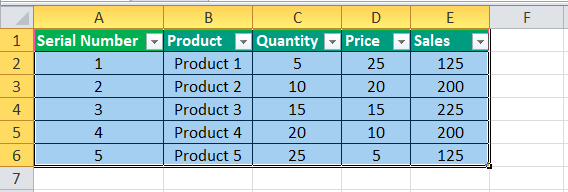
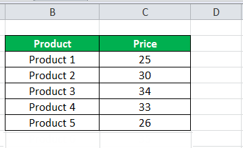
We have the following data,
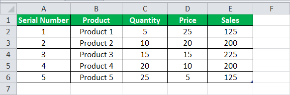
If we make a pivot table A Pivot Table is an Excel tool that allows you to extract data in a preferred format (dashboard/reports) from large data sets contained within a worksheet. It can summarize, sort, group, and reorganize data, as well as execute other complex calculations on it. read more with this normal data range from A1:E6, then if we insert a data in row 7, it will not reflect in the pivot table.
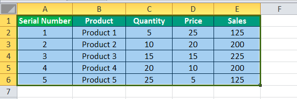
So we will first make a dynamic range.
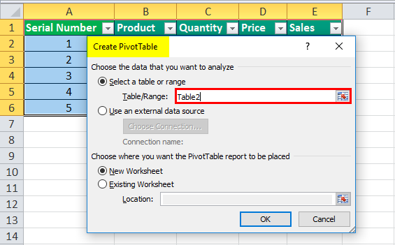
- Select the data, i.e., A1:E6.
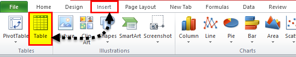
- In the Insert tab, click on Tables under the tables section.
- A dialog box pops up.
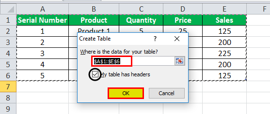
As our data has headers so remember to check on the box u201cMy Table has headersu201d and click ok.
- Our Dynamic Range is created.
- Select the data and in the Insert Tab under the excel tables section, click on pivot tables.
- As we have created the table, it takes a range as Table 2. Click on OK and in the pivot tables, Drag Product in Rows and Sales in Values.

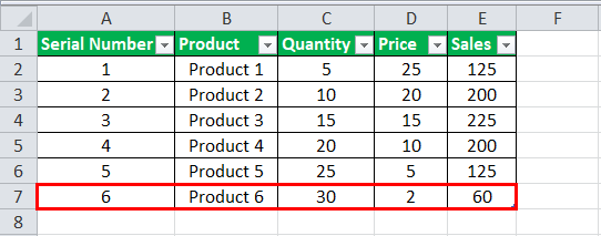
- Now in Sheet where we have our table insert Another Data in 7th
In the pivot table, refresh the pivot table.
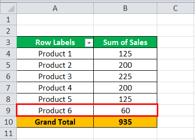
Our dynamic Pivot table has automatically updated data of Product 6 in the pivot table.
#2 – Using the OFFSET Function to create Dynamic Table in Excel
We can also use the OFFSET Function The OFFSET function in excel returns the value of a cell or a range (of adjacent cells) which is a particular number of rows and columns from the reference point. read more to create dynamic tables in excel. Let us have a look at one such example.
Example
I have a price list for my products which is I use for my calculations,
Select the data and give it a name
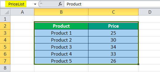
Now, whenever I refer to the data set pricelist, it will take me to the data in the range B2:C7, which has my price list. But if I update another row to the data, it will still take me to the range of B2:C7 because our list is static.
We will use the Offset Function to make the data range as dynamic.
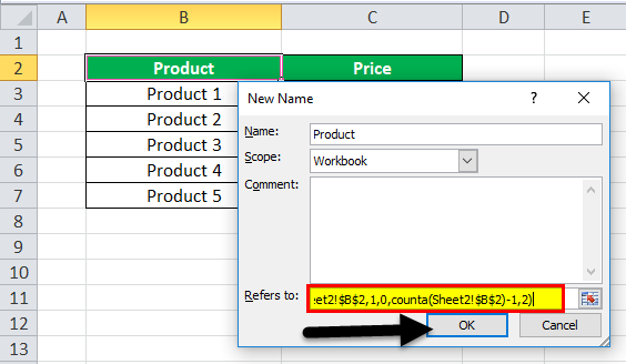
#1 – Under The Formulas Tab in the Defined Range, click on Defined Name, and a dialog box pops up.
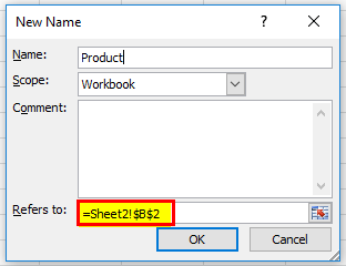
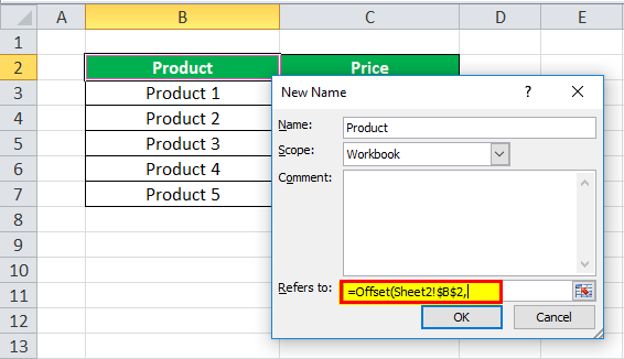
#2 – In the Name Box In Excel, the name box is located on the left side of the window and is used to give a name to a table or a cell. The name is usually the row character followed by the column number, such as cell A1. read more type in any name, I will use the PriceA. The scope is the current workbook, and currently, it is referring to the current cell selected, which is B2.
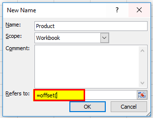
In Refers to write the following formula,
=offset(Sheet2!$B$2,1,0,counta(Sheet2!$B:$B)-1,2)
=offset(
#3 – Now select the starting cell, which is B2.
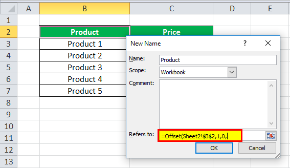
#4 – Now we need to type 1,0 as it will count how many rows or columns to go
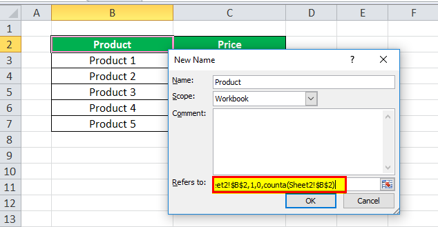
#5 – Now we need it to count whatever the data is in column B and use that as the number of rows, so use the COUNTA function The COUNTA function is an inbuilt statistical excel function that counts the number of non-blank cells (not empty) in a cell range or the cell reference. For example, cells A1 and A3 contain values but, cell A2 is empty. The formula "=COUNTA(A1,A2,A3)" returns 2. read more and select column B.
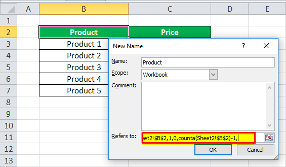
#6 – As we do not want the first Row, which is the product header, to be counted, so (-) 1 from it.
#7 – Now, the number of columns will always be two, so type 2 and click OK.
#8 – This data range won't be visible by default, so to see this, we need to click on Name Manager The name manager in Excel is used to create, edit, and delete named ranges. For example, we sometimes use names instead of giving cell references. By using the name manager, we can create a new reference, edit it, or delete it. read more under the Formula Tab and select Product,
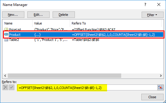
#9 – If we click on refers to it shows the data range,

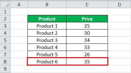
#10 – Now add another product in the table Product 6.
#11 – Now click on Product Table in the Name manager; it also refers to the new data inserted,

This is how we can use the Offset function to make a dynamic Tables.
Things to Remember
- Pivot Tables based on Dynamic range automatically get updated when refreshed.
- Using the offset function in Defined names can be seen from the Name Manager in the formula Tab.
Recommended Articles
This has been a guide to a Dynamic Tables in Excel. Here we discuss how to create a dynamic table in excel using TABLE and OFFSET Function along with practical examples and downloadable templates. You may learn more about excel from the following articles –
- Excel Merge Tables
- Pivot Table Sort
- Create a Dynamic Chart in Excel
- Create a Data Table in Excel
- 35+ Courses
- 120+ Hours
- Full Lifetime Access
- Certificate of Completion
LEARN MORE >>
How to Create a Dynamic Table in Excel
Source: https://www.wallstreetmojo.com/dynamic-tables-in-excel/